Navigate with Nav2 in hangar_sim

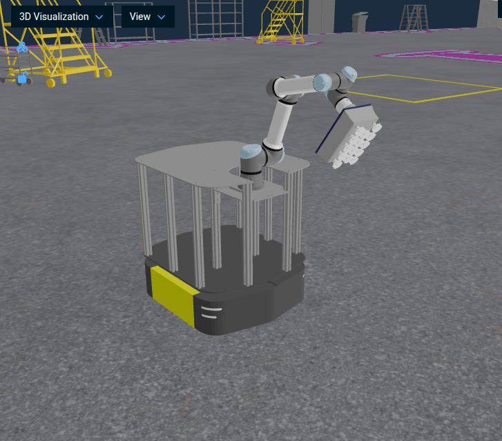
The hangar_sim robot configuration features a Clearpath Ridgeback mobile base carrying a UR5e arm. This guide covers the full mobile navigation stack: how the lidar feeds into Nav2's costmaps, how the robot localizes itself, how velocity commands reach the mecanum wheels, and how to use the navigation Objectives.

Adapting this to your own robot?

See Whole-Body Motion for configuring whole-body MoveIt planning with a mobile base, and Mobile Navigation Setup for wiring Nav2 into a new robot configuration package.

Launch the Runtime and Desktop App

We assume you have already installed MoveIt Pro to the default install location. Start the MoveIt Pro Runtime using:

moveit_pro run -c hangar_sim

Then launch or connect the separately distributed MoveIt Pro Desktop App. The Runtime does not serve a bundled user interface.

The Robot: Ridgeback Mecanum Base

Lidar Sensors

The robot is equipped with two SICK TIM571 planar lidars: one at the front bumper and one at the rear bumper.

Key characteristics:

• Each lidar sweeps 270° at ⅓° resolution — 811 beams, the TIM571's datasheet geometry — over a 0.05–25 m range, at 10 Hz
• Front lidar publishes scans to /scan_front; rear lidar publishes to /scan_rear, both with best-effort QoS
• Each scan passes through an independent angular bounds filter that clips chassis self-hits, removing the two rear-corner arcs at 0–31° and 239.5–270.5° (−0.01–0.54 rad and 4.18–4.72 rad) and keeping the roughly 208° in between
• Filtered scans are published on /scan_front_filtered and /scan_rear_filtered
• Combined coverage: 360° around the robot, with the two kept arcs overlapping to the sides

Both filtered topics are the obstacle sources for both costmaps.

How the scans are produced

Each scanner is simulated as a MuJoCo camera with DEPTH_TYPE=THREE_D_LIDAR, which picknik_mujoco_ros renders as depth tiles and stitches into an organized PointCloud2 on /lidar_front/points and /lidar_rear/points. The sweep is rendered on the render thread rather than measured inside mj_step, which is what lets it carry the full 811 beams without charging them to the physics step.

Localization and mapping need a LaserScan — slam_toolbox and amcl each accept exactly one scan topic and no point cloud — so lidar_flattener.py subscribes to both clouds and publishes the scans the rest of the stack reads. It takes the horizontal row of each cloud (the rows above and below it would put ceiling and floor returns into the scan plane), reverses it to the counter-clockwise LaserScan convention, and publishes /scan_front and /scan_rear spanning angle_min = 0 to angle_max = 4.7124 rad.

The scans are published in the lidar_front_ROS and lidar_rear_ROS frames, which robot_drivers_to_persist_sim.launch.py broadcasts as static transforms on ridgeback_base_link at ±0.45 m along X and 0.15 m up. Each is z-up with its X axis at the scan's angle_min, so a beam's index maps directly to a bearing on the robot. The clouds themselves are published in lidar_front_optical_frame and lidar_rear_optical_frame, which are there for RViz and tooling; nothing in the navigation stack reads them.

Localization

By default, hangar_sim runs beluga_amcl for map-based localization. AMCL matches a merged 360° lidar scan — the front and rear scans combined into /scan_merged — against a pre-built map to estimate the robot's pose, publishing the map→odom transform that anchors the odometry frame to the map. The scans are merged because the front lidar alone gives the particle filter too little structure near the long hangar fuselage, where it can otherwise lose track. Because the Ridgeback is a mecanum (omnidirectional) base, AMCL uses an omnidirectional motion model so that lateral motion is not mistaken for rotation. Localization is configured in the amcl section of nav2_params.yaml.

Set localization:=False in robot_drivers_to_persist_sim.launch.py to disable AMCL; the launch then publishes a static map→odom transform instead, falling back to passing odometry straight through to Nav2.

warning

With AMCL disabled, the robot relies on odometry alone. On a real robot the position estimate then drifts over time due to wheel slip and IMU bias; over medium to long distances this drift accumulates, causing the costmap and planned paths to diverge from the robot's actual position. Keep map-based localization enabled for real-robot deployments.

Underneath AMCL, hangar_sim ships with an optional Fuse state estimator that fuses two sensor sources for a more realistic odometry estimate:

• Wheel odometry from /platform_velocity_controller_nav2/odom — provides x/y position and yaw, fused differentially to handle drift
• IMU from /imu_sensor_broadcaster/imu_reliable — provides absolute orientation (roll, pitch, yaw) and yaw rate, anchoring the estimate against wheel slip

The filtered estimate is published on /odom_filtered. To enable it, set use_fuse to true in robot_drivers_to_persist_sim.launch.py and update odom_topic in nav2_params.yaml from /odom to /odom_filtered.

The video below shows Fuse in action during straight, spin, strafe, and straight maneuvers. The green arrow is raw wheel odometry (drifting), the red arrow is ground truth from MuJoCo, and the yellow path is the Fuse-filtered estimate tracking the ground truth closely.

Costmaps

Nav2 maintains two costmaps simultaneously. Both read obstacle data from /scan_front_filtered and /scan_rear_filtered as independent observation sources.

Global Costmap

The global costmap covers the full hangar map and is used for high-level path planning.

Property	Value
Frame	map
Resolution	5 cm/cell
Update frequency	1 Hz
Layers	Static (pre-built map) + Obstacle (front + rear lidar, 8.0 m max range) + Inflation (0.7 m radius)

The static layer loads the pre-built occupancy grid of the hangar. The obstacle layer adds dynamic obstacles from both lidars, up to 8.0 m range (with 10.0 m raytrace for clearing). The inflation layer expands all obstacles by 0.7 m, approximately the robot radius plus padding, to ensure the robot body clears obstacles while traversing.

Why limit obstacle range to 8.0 m when the lidar reaches farther?

A few reasons drive this choice:

• Long-range lidar returns tend to be noisier, so capping the obstacle range filters out unreliable readings at the edges of the sensor's range.
• Restricting the range limits how much of the hangar scene is visible to the costmap, keeping costmap updates more focused and easier to observe in tutorials.
• The raytrace range (10.0 m) is intentionally set longer than the obstacle range (8.0 m). This avoids a common edge case where a beam that just misses a real obstacle fails to clear a previously marked cell, leaving a phantom obstacle stuck in the costmap.

Local Costmap

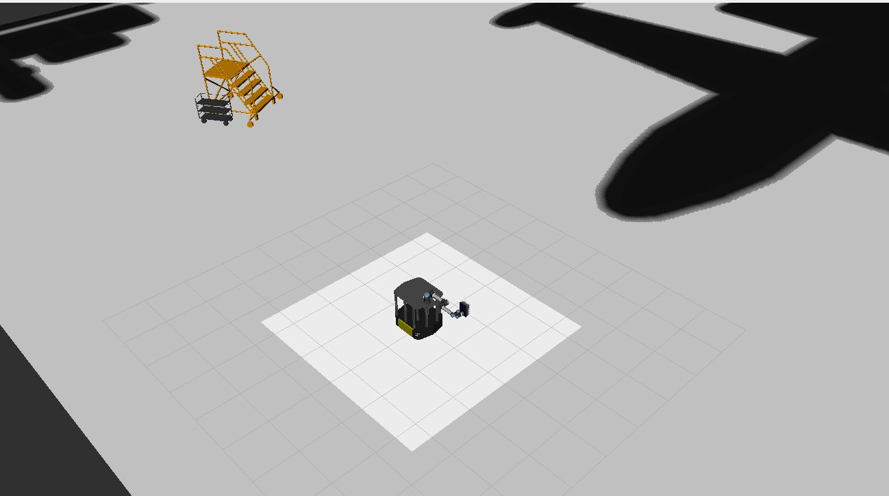
The local costmap is a 5 × 5 m rolling window centered on the robot, used for reactive obstacle avoidance during path following. In hangar_sim, the lidar is primarily a long-range planar sensor suited for localization; the local costmap here demonstrates the concept but does not include the short-range sensors (such as depth cameras) that would typically drive its size in a production system.

Property	Value
Frame	odom
Size	5 × 5 m rolling window
Resolution	5 cm/cell
Update frequency	10 Hz
Layers	Obstacle (front + rear lidar, 4.5 m raytrace range, 3.5 m obstacle range) + Inflation (0.75 m radius)

The local costmap updates at 10 Hz (much faster than the global costmap) and marks obstacles up to 3.5 m away, with a 4.5 m raytrace range for clearing. It does not include a static layer; the robot's immediate surroundings are treated as fully dynamic.

Costmaps in the MoveIt Pro Desktop App

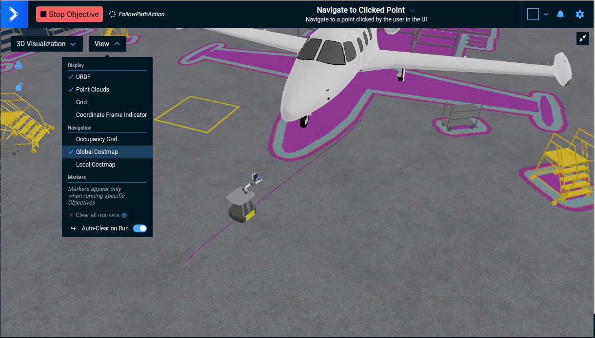
Both costmaps are visible in the Visualization view as colored overlays in the 3D scene. The UI subscribes to the costmap topics published by Nav2 and updates in real time as the robot moves and new obstacles are detected.

To enable the costmap overlays, open the View menu and toggle Global Costmap and/or Local Costmap under the Navigation section.

Footprint overlays

Required Version

This feature requires MoveIt Pro version 9.5 or newer.

The same Navigation section also exposes Local Footprint (light green) and Global Footprint (cyan) toggles that overlay the robot footprint published by each costmap. Local and global footprints are rendered separately because each costmap can apply different inflation, so the two outlines do not always coincide. The footprint topics default to /local_costmap/published_footprint and /global_costmap/published_footprint; they are configurable through the nav2LocalFootprintTopic and nav2GlobalFootprintTopic keys in the frontend settings.

The RViz view below illustrates the 5×5 m rolling window size — the white square is the local costmap centered on the robot, surrounded by the black global costmap.

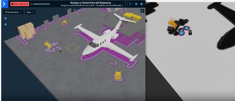
The side-by-side below shows the MoveIt Pro Desktop App (left) with the purple inflation overlay around detected obstacles, alongside RViz (right) displaying the local costmap updating over the black global costmap with white lidar hit points from both the front and rear sensors.

Sensor overlays

Required Version

This feature will not be released until MoveIt Pro version 10.2.

To inspect the sensor data behind the navigation map, open View, enable Sensor Streaming under Display, and enable the sources you want to compare. The 3D Visualizer discovers live sensor_msgs/PointCloud2 and sensor_msgs/LaserScan topics. In hangar_sim, useful sources include the front and rear lidar point clouds and the filtered laser scans used by the costmaps.

Expand a source's settings to adjust its Point Size in meters. Leave Use Source Colors enabled to preserve colors supplied by the sensor; sources without color data appear orange so they remain visible against the map. Disable it to select a solid color for that source. Visibility and style preferences are saved in your browser, and changing a style updates the live display without restarting the stream. Disabling a source stops its streaming subscription.

Set the 3D Visualizer's Fixed Frame to map to compare the sensor returns with the navigation map. The Runtime transforms scan returns using their acquisition times before streaming them, so a moving sensor does not drag a previous scan through the scene. Invalid and out-of-range returns are omitted. If the required transforms are unavailable, new scan data is withheld rather than placed using an unrelated latest transform.

Particle filter overlay

When a localization node publishes a geometry_msgs/msg/PoseArray on a topic whose final segment contains "particle" (e.g. /particlecloud from nav2 AMCL and beluga, /particle_cloud, or namespaced variants like /robot_2/particlecloud), the View menu lists it under Navigation as Particle Filter - topic. Enable the topic to overlay magenta arrows at every candidate pose. The arrow positions and headings update with the particle cloud, so the distribution spreads when localization uncertainty grows and contracts as the filter converges.

Controller Pipeline

At startup, joint_trajectory_controller (whole-body) is the active controller. When a navigation Objective runs, the SwitchController Behavior deactivates it and activates platform_velocity_controller_nav2. The Nav2 command pipeline then works as follows:

1. MPPI controller (FollowPath) — runs at 20 Hz, samples trajectory candidates and selects the one with the lowest cost against the costmaps
2. Velocity smoother — smooths the MPPI output to respect acceleration limits (max ±2.5 m/s²)
3. /cmd_vel relay — forwards /cmd_vel to /platform_velocity_controller_nav2/cmd_vel_unstamped
4. platform_velocity_controller_nav2 — a clearpath_mecanum_drive_controller controller that converts the body-frame velocity command to individual wheel speeds for the four mecanum wheels

note

Running a whole-body arm Objective (for example, Teleoperate) switches back to joint_trajectory_controller, displacing platform_velocity_controller_nav2. Navigation Objectives re-activate it via SwitchController at the start of each run.

Navigating the Robot

Navigate to Clicked Point

The simplest navigation Objective. Select it from the Objectives panel to get started.

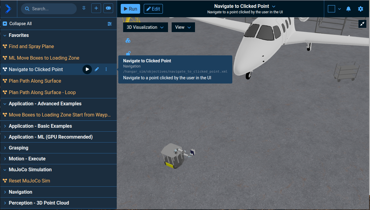
It then:

1. Re-seeds AMCL localization at the robot's current pose with SetInitialPose, so each run starts from a clean position estimate
2. Computes a single global path to the user-clicked goal using ComputePathToPoseAction
3. Displays the planned path and waits for user confirmation with WaitForUserPathApproval
4. Follows the approved path using FollowPathAction

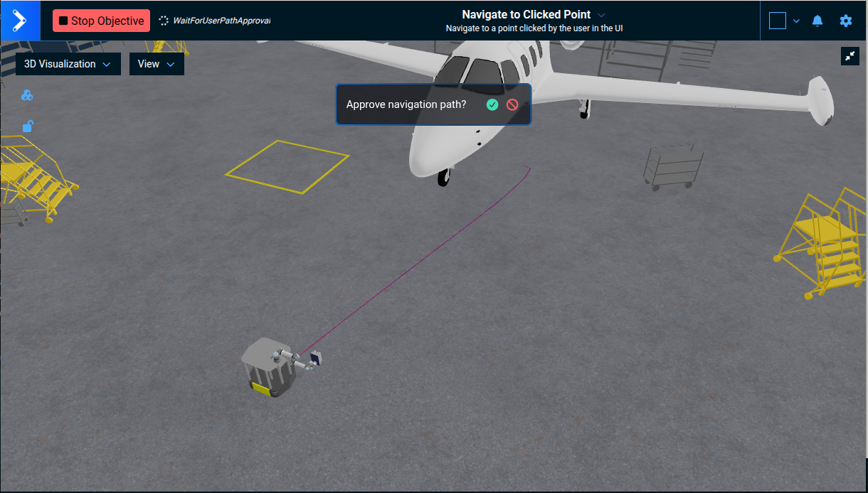
If an obstacle appears during execution, the robot may get stuck — there is no replanning, and the Objective will keep running until you click Stop Objective.

Navigate to Clicked Point with Replanning

For dynamic environments where obstacles may appear during navigation, use Navigate to Clicked Point with Replanning. This Objective delegates full navigation control to Nav2, which replans the path continuously as the local costmap updates.

See Navigate to a Goal with Replanning for a detailed walkthrough of how this Objective works, how Nav2's replanning Behavior Tree handles recovery, and when you may need to stop the Objective manually.