Cartesian Trapezoidal Velocity Profile
Package: path_ik (trajectory_utils.hpp/.cpp) Author: Mario Prats Date: 2026-04-16
Table of Contents
- 1. Problem Statement
- 2. Inputs and Outputs
- 3. Challenges
- 3.1. Mixed Translation/Rotation Paths
- 3.2. Joint-Space Feasibility
- 4. Mathematical Foundation
- 4.1. Path Distances
- 4.2. Rate-Limited Arc Length
- 4.3. Effective Acceleration
- 4.4. Trapezoidal Profile Construction
- 4.5. Timestamp Assignment
- 4.6. Joint-Space Feasibility Check
- 4.7. Resampling at Control Rate
- 5. Algorithm Summary
- 6. Implementation
- 6.1. Data Types
- 6.2. Function Signature
- 6.3. Internal Helpers
- 6.4. Integration with Existing Code
- 7. Edge Cases
- 8. Testing Strategy
- 9. Future Extensions
1. Problem Statement
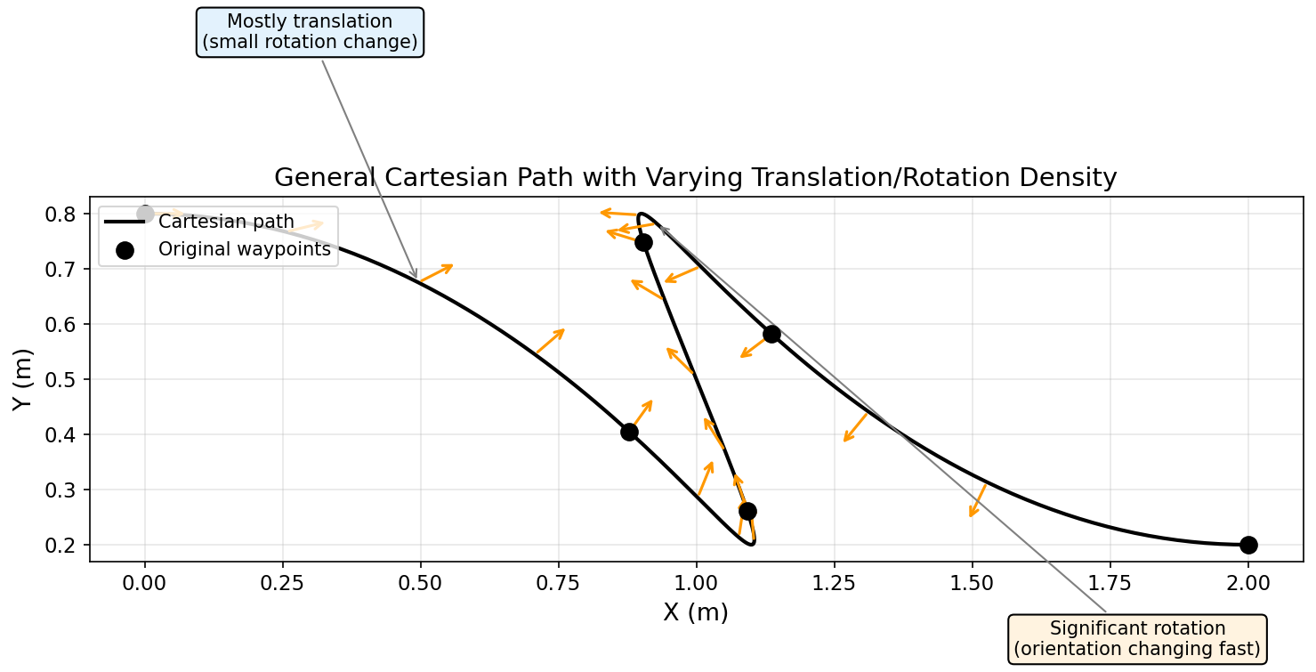
We have a dense Cartesian-space path (a sequence of 6-DOF poses representing both translation and orientation) and a corresponding dense joint-space path (the result of calling pathIK, which computes the incremental inverse kinematics with blending at intermediate waypoints). Both paths have the same number of waypoints and are geometrically aligned: waypoint i of the joint path is the IK solution for waypoint i of the Cartesian path.
The goal is to time this path — i.e., assign a timestamp to every waypoint — so that the resulting trajectory follows a trapezoidal velocity profile in Cartesian space:
- Accelerate from rest to the desired Cartesian velocity.
- Cruise at the desired Cartesian velocity.
- Decelerate from the desired Cartesian velocity to rest.
The trajectory must also respect joint-space velocity and acceleration limits. If it cannot (e.g., near a kinematic singularity where small Cartesian motion requires large joint motion), the function must fail and report a time-dilation factor that tells the caller how much to relax the Cartesian limits to make the trajectory feasible.
2. Inputs and Outputs
Inputs:
| Parameter | Type | Description |
|---|---|---|
| cartesian_path | Path (std::vector<Eigen::Isometry3d>) | Dense sequence of N 6-DOF poses |
| joint_path | JointSpacePath (std::vector<Eigen::VectorXd>) | Dense sequence of N joint-space waypoints (from pathIK) |
| cartesian_limits | CartesianLimits | Max translational velocity/acceleration and max rotational velocity/acceleration |
| max_joint_velocities | Eigen::VectorXd | Per-joint velocity limits (rad/s) |
| max_joint_accelerations | Eigen::VectorXd | Per-joint acceleration limits (rad/s^2) |
| control_rate | int | Trajectory sampling rate in Hz |
Output (success): ResampledTrajectory — uniformly sampled at control_rate, containing timestamps plus joint positions, velocities, and accelerations for each sample.
Output (failure): TrapezoidalProfileError — contains the required time-dilation factor alpha and diagnostic information about which limit was the bottleneck.
3. Challenges
3.1. Mixed Translation/Rotation Paths
The Cartesian path is not a single straight line — it is a general sequence of poses with blending at intermediate waypoints. The ratio of translational to rotational motion varies along the path: some segments may be mostly translational (the tool moves but barely rotates), while others may be mostly rotational (the tool reorients in place).
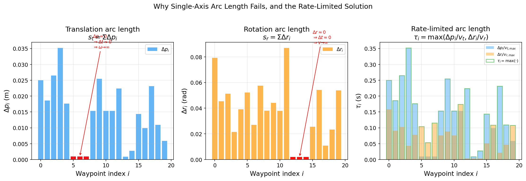
This means we cannot parameterize the path by translation arc length alone. If a segment has near-zero translation but significant rotation, the translational arc length increment is near zero, meaning the time allocated to that segment would be near zero, causing the rotational velocity to spike to infinity.
The same problem occurs in reverse if we parameterize by rotation arc length — pure-translation segments would get near-zero time.
3.2. Joint-Space Feasibility
Even when the Cartesian velocity profile is well-formed, the resulting joint-space velocities and accelerations may exceed the robot's limits. This is especially common near kinematic singularities, where small Cartesian displacements map to large joint motions through the Jacobian.
The requirement is strict: if joint limits are violated, the trajectory is infeasible and must be rejected. The function should not silently slow down locally (which would break the trapezoidal shape) — instead, it should report failure with a time-dilation factor so the caller can retry with relaxed Cartesian limits.
4. Mathematical Foundation
4.1. Path Distances
For each consecutive pair of waypoints (i, i+1) in the Cartesian path, compute:
Translational distance:
where p_i is the translation component of the i-th pose (Euclidean norm).
Rotational distance:
where R_i is the rotation component of the i-th pose, and log is the logarithmic map from SO(3) to so(3), yielding an axis-angle vector whose norm is the rotation angle. This is equivalent to the geodesic distance on SO(3).
Implementation note: Use path_ik::poseError() which returns a 6D vector [Dp_x, Dp_y, Dp_z, Dr_x, Dr_y, Dr_z]. The translational distance is the norm of the first 3 components, and the rotational distance is the norm of the last 3 components.
4.2. Rate-Limited Arc Length
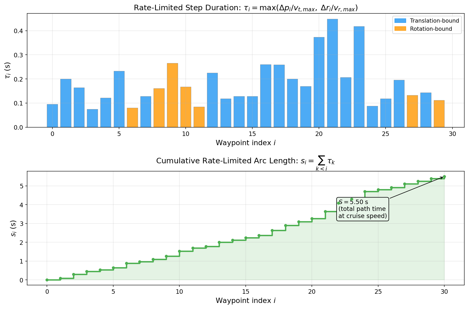
The core insight of this design. Define the rate-limited step duration at each step as the minimum time needed to traverse that step without violating either Cartesian velocity limit:
where v_t_max is the maximum translational velocity (m/s) and v_r_max is the maximum rotational velocity (rad/s).
The cumulative rate-limited arc length is:
Units: tau_i and s_i have units of seconds. S represents the total time the path would take if the robot could cruise at full speed the entire time (no acceleration/deceleration phase).
Key properties:
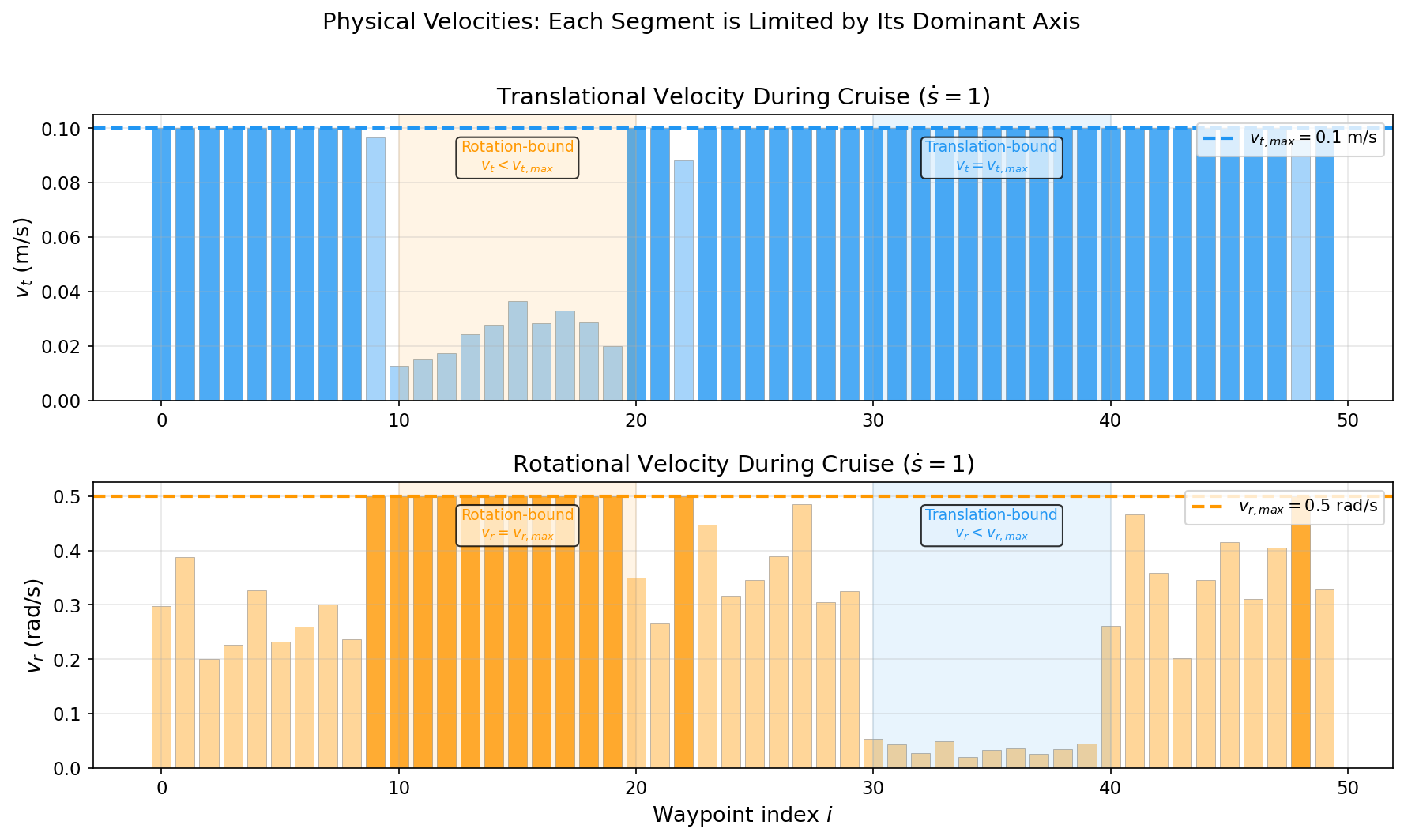
- Translation-bound segments (Dp_i / v_t_max >= Dr_i / v_r_max): tau_i = Dp_i / v_t_max. The translational velocity reaches v_t_max during cruise, while the rotational velocity stays below v_r_max.
- Rotation-bound segments (Dr_i / v_r_max > Dp_i / v_t_max): tau_i = Dr_i / v_r_max. The rotational velocity reaches v_r_max during cruise, while the translational velocity stays below v_t_max.
- Pure translation (Dr_i = 0): tau_i = Dp_i / v_t_max. Degenerates to standard translational arc length parameterization.
- Pure rotation (Dp_i = 0): tau_i = Dr_i / v_r_max. Degenerates to standard rotational arc length parameterization.
Velocity guarantee: During cruise (when the profile speed s_dot = 1), the physical velocities at step i are:
Both limits are respected at every step, by construction.
4.3. Effective Acceleration
The trapezoidal profile on s has a scalar acceleration s_ddot during the ramp phases. This maps to physical accelerations at each waypoint:
We need a_t(i) <= a_t_max and a_r(i) <= a_r_max at every waypoint in the acceleration/deceleration phases. Since Dp_i / tau_i <= v_t_max and Dr_i / tau_i <= v_r_max (by construction of tau_i), the following conservative bound is always feasible:
Units: a_eff has units of 1/s (because s has units of seconds).
Proof of feasibility: At any waypoint i:
- a_t(i) = (Dp_i / tau_i) * a_eff <= v_t_max * (a_t_max / v_t_max) = a_t_max ✓
- a_r(i) = (Dr_i / tau_i) * a_eff <= v_r_max * (a_r_max / v_r_max) = a_r_max ✓
Note on conservatism: This bound is tight when the same axis binds everywhere. It is slightly conservative when translation binds at some waypoints and rotation at others — in that case, the per-waypoint bound a_eff(i) = min(a_t_max * tau_i / Dp_i, a_r_max * tau_i / Dr_i) would be tighter. However, using min_i a_eff(i) complicates the profile (the acceleration depends on where you are), and the conservatism in practice is small. The closed-form expression is preferred for simplicity and correctness.
4.4. Trapezoidal Profile Construction
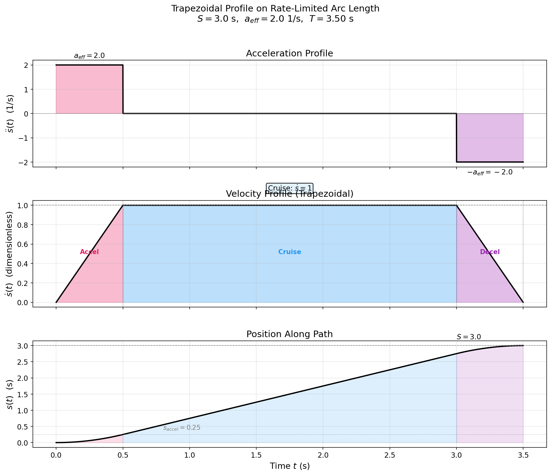
With S (total arc length in seconds), cruise speed v = 1 (dimensionless), and acceleration a_eff (1/s), the profile s_dot(t) is:
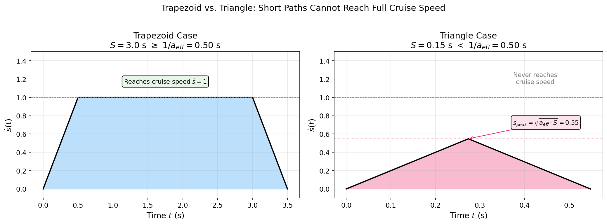
Case 1: Trapezoid (path long enough to reach cruise speed)
Condition: 2 * s_accel <= S where s_accel = v^2 / (2 * a_eff) = 1 / (2 * a_eff)
Case 2: Triangle (path too short to reach cruise speed)
Condition: 2 * s_accel > S
4.5. Timestamp Assignment
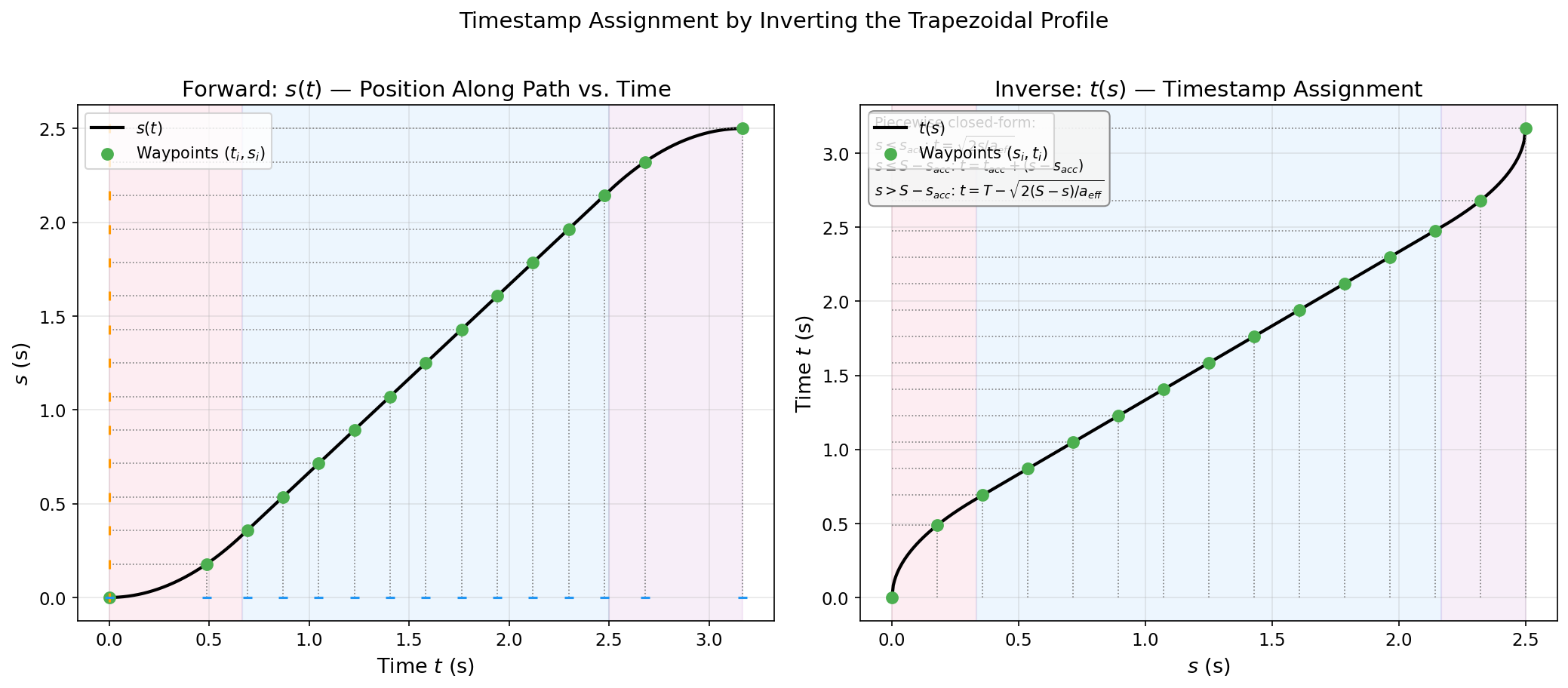
Given the cumulative arc length s_i for each waypoint, invert the profile s(t) to obtain the timestamp t_i = t(s_i):
Trapezoid case:
Triangle case:
All inversions are closed-form — no numerical root finding needed.
4.6. Joint-Space Feasibility Check
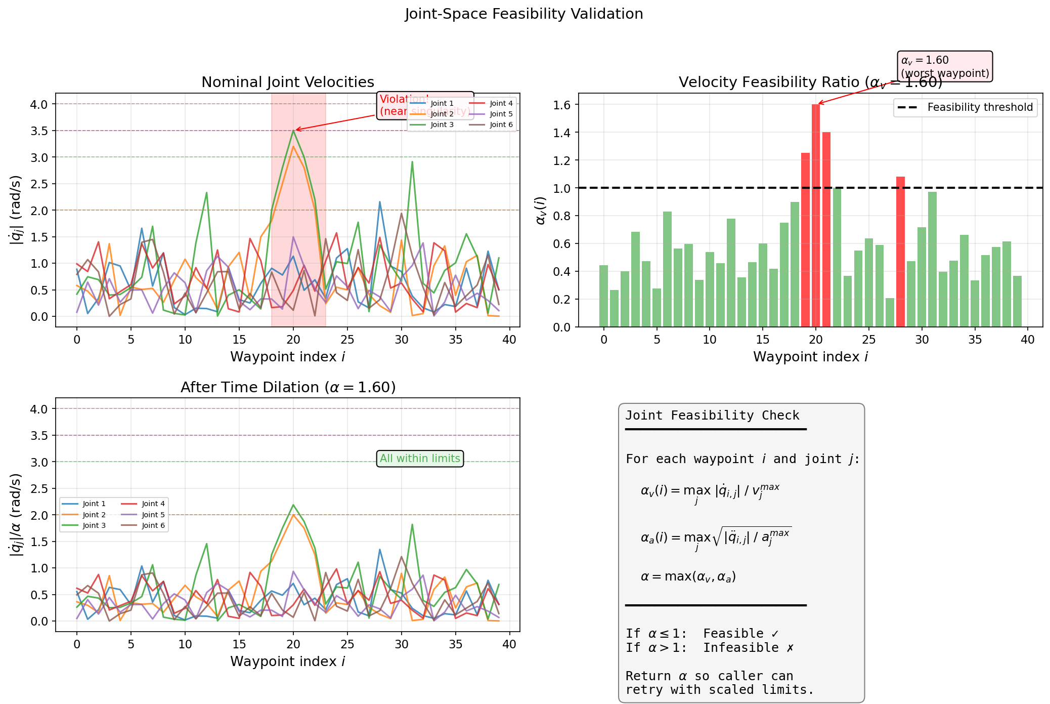
After assigning timestamps, verify that the resulting joint-space velocities and accelerations are within limits. Compute joint derivatives analytically using the chain rule:
where:
- ‘q`(s_i)≈(q_{i+1} - q_{i-1}) / (s_{i+1} - s_{i-1})— central finite difference of joint positions with respect tos -q''(s_i)≈(q'_{i+1} - q'_{i-1}) / (s_{i+1} - s_{i-1})— central finite difference ofq'(s) -s_dotands_ddotare known analytically from the trapezoidal profile at eachs_i`
Advantages of analytical derivatives over finite differences in time:
- The feasibility check decouples from the resampling step.
- The reported alpha is exact (not affected by resampling resolution).
- The failure path is cheap — no need to construct the full resampled trajectory.
Computing the time-dilation factor:
- If alpha <= 1: feasible. Proceed to resampling.
- If alpha > 1: infeasible. Return an error with alpha and bottleneck information.
Why alpha_a uses sqrt: Under time dilation by factor alpha, velocities scale as 1/alpha and accelerations scale as 1/alpha^2. So to bring the worst-case acceleration within limits, you need alpha >= sqrt(violation_ratio).
What the caller can do with alpha: Retry with v_t_max / alpha, v_r_max / alpha, a_t_max / alpha^2, a_r_max / alpha^2. This preserves the trapezoidal shape and makes the trajectory alpha times longer.
4.7. Resampling at Control Rate
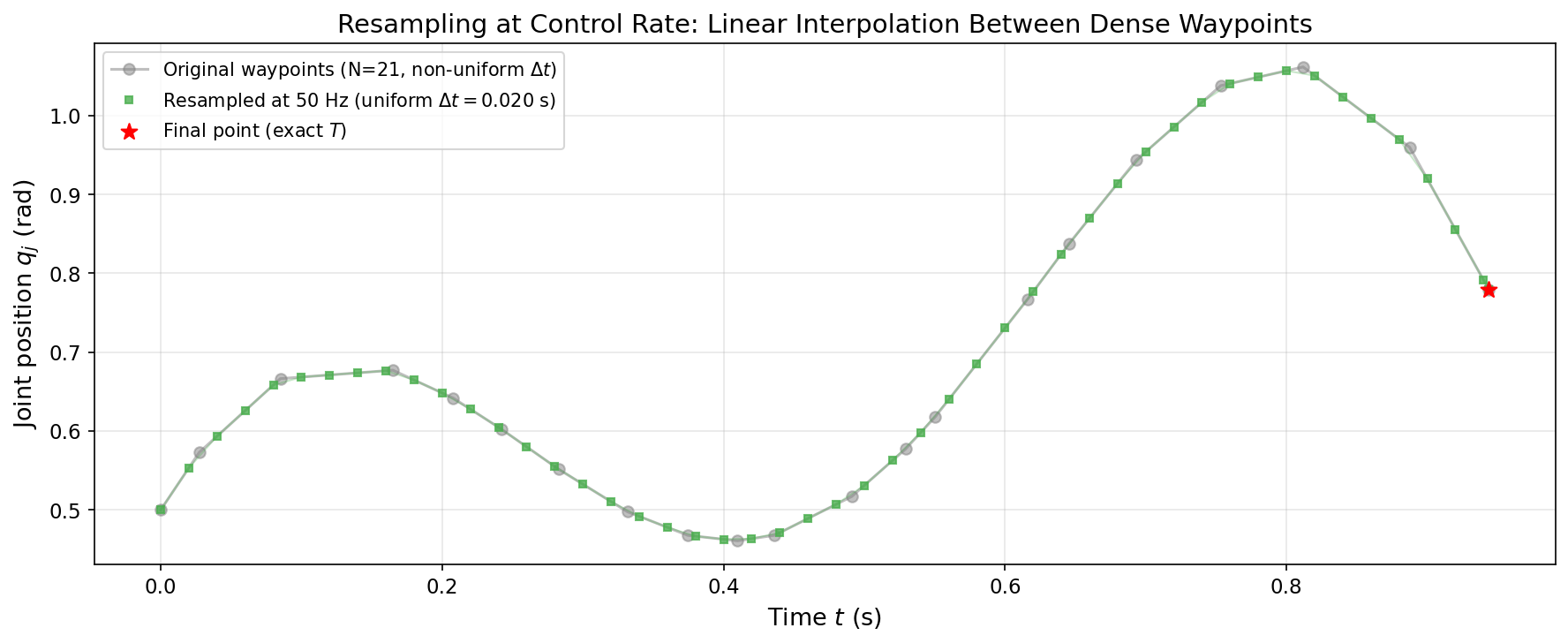
The output trajectory must be uniformly sampled at control_rate Hz. Joint velocities and accelerations must be computed analytically from the trapezoidal profile, not via finite differences of resampled positions.
Why not finite differences?
The pathIK output has approximately uniform spatial density (~1mm per waypoint). Under the trapezoidal profile, this maps to non-uniform temporal density: during acceleration/deceleration the robot moves slowly, so each spatially-uniform waypoint spans a large time interval; during cruise, waypoints are densely packed in time.
If we resample positions at a uniform control rate and then compute velocities via finite differences, the result exhibits a staircase pattern: within each original waypoint pair, linear interpolation produces constant velocity, which then jumps at the pair boundary. This artifact is most visible during the accel/decel phases where a single original waypoint pair can span many resampled control steps.
Arc-length-based interpolation with analytical derivatives
The solution is to work in arc-length space using the forward profile s(t), and compute velocities and accelerations analytically from the chain rule.
Forward profile — given time t, compute (s, ṡ, s̈):
Trapezoid case:
Resampling procedure:
For each control-rate sample k = 0, 1, ..., floor(T / dt) at time t_k = k * dt:
- Evaluate the forward profile at t_k to get (s_k, ṡ_k, s̈_k).
- Find the bracketing original waypoints i such that s_i <= s_k < s_{i+1} (monotone scan in arc-length space, O(N) total).
- Interpolate position in arc-length space:
frac = (s_k - s_i) / (s_{i+1} - s_i)q_k = q_i + frac * (q_{i+1} - q_i)
- Interpolate joint derivatives at s_k:
q'_k = q'_i + frac * (q'_{i+1} - q'_i)q''_k = q''_i + frac * (q''_{i+1} - q''_i)
- Compute analytical velocity:
q_dot_k = q'_k * s_dot_k
- Compute analytical acceleration:
q_ddot_k = q''_k * s_dot_k^2 + q'_k * s_ddot_k
If |floor(T / dt) * dt - T| >= 1e-9, append a final sample at exactly T. Set endpoint velocities and accelerations to exactly zero (the profile starts and ends at rest).
Key properties of this approach:
- Velocities are smooth by construction. They come from ‘q`(s) · ṡ(t), whereṡ(t)is the continuous trapezoidal profile andq'(s)is interpolated from the dense path. No finite-difference staircase artifacts.
- **Accelerations reflect the profile exactly.** Thes̈term produces the correct constant acceleration during the ramp phases, and theq''(s) · ṡ²term captures path-curvature effects.
- **The joint-space feasibility check (Step 7) and the resampling (Step 8) use the same chain-rule formulas**, ensuring consistency between what was validated and what is output.
- **Position interpolation in arc-length space** is equivalent to interpolating in time for straight segments, but is better-conditioned during accel/decel because the original waypoints are uniformly spaced ins(not int`).
Why linear interpolation of positions is still sufficient: The input path is already dense (from pathIK with sub-millimeter/sub-milliradian step sizes). Adjacent waypoints are very close in joint space, so linear interpolation between them introduces negligible position error. The smoothness improvement comes entirely from computing velocities and accelerations analytically rather than from finite differences.
5. Algorithm Summary
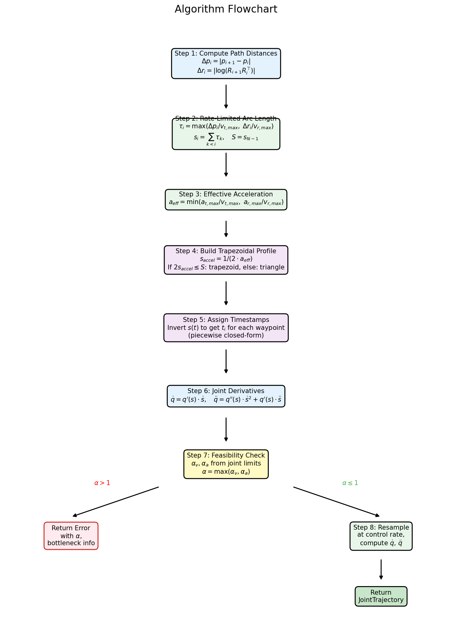
Step 1 — Path distances. Compute Dp_i and Dr_i for each consecutive pair of Cartesian waypoints.
Step 2 — Rate-limited arc length. Compute tau_i = max(Dp_i / v_t_max, Dr_i / v_r_max) and cumulative s_i = sum tau_k. Total path cost: S = s_{N-1}.
Step 3 — Effective acceleration. Compute a_eff = min(a_t_max / v_t_max, a_r_max / v_r_max).
Step 4 — Trapezoidal profile. Compute s_accel = 1 / (2 * a_eff). If 2 * s_accel <= S, use trapezoid; otherwise triangle. Compute total duration T.
Step 5 — Timestamp assignment. For each waypoint, invert s(t) to get t_i using the piecewise closed-form inverse.
Step 6 — Joint derivatives. Compute ‘q`(s)andq''(s)via central finite differences. Computeq_dotandq_ddot` analytically from the chain rule.
Step 7 — Feasibility check. Compute alpha_v, alpha_a, and alpha = max(alpha_v, alpha_a). If alpha > 1, return TrapezoidalProfileError with alpha and bottleneck info. Otherwise proceed.
Step 8 — Resample. For each control-rate sample time, evaluate the forward profile to get (s, ṡ, s̈), interpolate joint positions in arc-length space, and compute velocities and accelerations analytically via ‘q̇ = q`(s)·ṡandq̈ = q''(s)·ṡ² + q'(s)·s̈`. Append exact final point if needed.
Step 9 — Return. Return ResampledTrajectory.
6. Implementation
6.1. Data Types
6.2. Function Signature
6.3. Internal Helpers
The implementation should be decomposed into small, testable pure functions:
6.4. Integration with Existing Code
- path_ik::poseError() (math.hpp): Use for computing Dp_i and Dr_i. Returns a 6D vector; take the norm of the first 3 components for translational distance, and the norm of the last 3 for rotational distance.
- path_ik::Path and path_ik::JointSpacePath (types.hpp): Existing type aliases for std::vector<Eigen::Isometry3d> and std::vector<Eigen::VectorXd>.
- trajectory_utils.hpp: Add the new function and types alongside the existing createTrajectoryFromWaypoints. The existing function uses TOTG (Time-Optimal Trajectory Generation) which operates in joint space; the new function enforces a Cartesian-space velocity profile, which is a fundamentally different contract.
- appendToTrajectoryMessage() (trajectory_utils.cpp): The resampling step can follow the same pattern (reserve, add points with time_from_start, handle final point) but operates on the non-uniform timestamps rather than a Trajectory object.
7. Edge Cases
| Case | Behavior |
|---|---|
| cartesian_path.size() != joint_path.size() | Return error: mismatched path sizes. |
| cartesian_path.size() < 2 | Return error: path must have at least 2 waypoints. |
| Dp_i = 0 and Dr_i = 0 for some step | Skip the step (duplicate waypoint). Log a warning if this happens. |
| Dp_i = 0 for all steps (pure rotation path) | Works correctly: tau_i = Dr_i / v_r_max, profile parameterized by rotation. |
| Dr_i = 0 for all steps (pure translation path) | Works correctly: tau_i = Dp_i / v_t_max, degenerates to translational arc length. |
| S = 0 (all waypoints identical) | Return error: zero-length path. |
| Path too short for trapezoid | Triangle profile used automatically. v_peak < 1. No error — this is a valid profile. |
| Joint limits violated | Return TrapezoidalProfileError with alpha > 1. |
| control_rate <= 0 | Return error: invalid control rate. |
| Negative or zero Cartesian limits | Return error: invalid limits. |
| Joint velocity/acceleration vector size mismatch | Return error: dimension mismatch. |
| max_joint_velocities or max_joint_accelerations has zero or negative entries | Return error: invalid joint limits. |
8. Testing Strategy
All internal helpers are pure functions, making them ideal for unit testing without any ROS infrastructure.
Unit tests (pure functions, no ROS):
| Test Category | What to Test |
|---|---|
| computePathDistances | Straight-line path (known distances), pure rotation, pure translation, single segment, identical waypoints. |
| computeRateLimitedArcLength | Translation-dominant, rotation-dominant, mixed, pure-rotation (Dp=0), pure-translation (Dr=0). |
| computeEffectiveAcceleration | Translation-limited, rotation-limited, equal limits. |
| buildTrapezoidalProfile | Trapezoid case, triangle case, boundary (exactly 2*s_accel = S). |
| invertProfile | All three phases (accel, cruise, decel), boundary values (s=0, s=S), triangle case. |
| assignTimestamps | Monotonicity of timestamps, t_0 = 0, t_{N-1} = T. |
| checkJointFeasibility | Feasible case (alpha <= 1), infeasible velocity, infeasible acceleration, worst-waypoint reporting. |
| resampleTrajectory | Uniform spacing, final point inclusion, velocity/acceleration at endpoints = 0. |
| End-to-end | Straight-line path with known analytical solution, verify Cartesian velocity is trapezoidal, verify joint limits respected. |
Error path tests:
| Condition | Expected Error |
|---|---|
| Mismatched path sizes | Descriptive error message |
| Empty path | Descriptive error message |
| Zero Cartesian velocity | Descriptive error message |
| Joint limit violation | TrapezoidalProfileError with alpha > 1, correct bottleneck joint/waypoint |
Adversarial tests:
| Scenario | What it Catches |
|---|---|
| Path with one near-singular waypoint | Verifies alpha is computed from the worst waypoint, not averaged |
| Path where alpha_v and alpha_a differ | Verifies the correct max is taken |
| Very short path (2 waypoints) | Triangle profile edge case |
| Path with large rotation but tiny translation | Verifies rotation-bound behavior |
9. Future Extensions
- TOPP-RA integration. If the global feasibility check (pass/fail) proves too conservative in practice — e.g., one waypoint near a singularity forces the entire trajectory to slow down — consider adding a TOPP-RA mode that locally adjusts s_dot while respecting all constraints. This changes the contract (profile is no longer a pure trapezoid) and should be a separate function or an opt-in mode.
- Anisotropic Cartesian limits. The current design uses scalar limits (v_t_max, v_r_max). If per-axis limits are needed (different max velocity in X vs Z), the tau_i computation would use max(|Dp_{i,x}| / v_x_max, |Dp_{i,y}| / v_y_max, |Dp_{i,z}| / v_z_max, ...).
- Tighter effective acceleration. Replace the conservative a_eff = min(a_t_max/v_t_max, a_r_max/v_r_max) with the per-waypoint minimum min_i min(a_t_max * tau_i / Dp_i, a_r_max * tau_i / Dr_i). This yields a tighter bound but requires a pass over all waypoints during profile construction.
- Multi-segment trajectories. Support stitching multiple trapezoidal segments (e.g., accelerate to v1, then change to v2 at a waypoint, then decelerate), using the appendToTrajectoryMessage pattern already in the codebase.
- Trajectory blending. When blending two trajectories (the reason this function is being developed), the trapezoidal profile may need to start or end at a non-zero velocity. Extend the profile to support v_start != 0 and/or v_end != 0.
Generated via doxygen2docusaurus 2.2.2 by Doxygen 1.9.8.